Shrink a voice clip 142× smaller — and still understand it

00Try it on your own voice

Hit Start recording, say a sentence or two (up to 6 seconds), then stop. The model runs entirely in your browser — your voice is never uploaded anywhere. Pick a quality level to choose how much you compress: lower quality = much smaller file size.

01Pre-recorded examples

Six clips of real human speech (from the LibriSpeech audiobook dataset), each compressed and rebuilt at three quality levels. Hit play on each version to hear the trade-off — the lowest quality is about 568× smaller than the original.

02Training curves

All four signals logged every 25 steps. Reconstruction L1 in the time domain, multi-scale STFT loss across the frequency domain, VQ commitment loss, and held-out SI-SDR at full bitrate.

03Spectrogram comparison

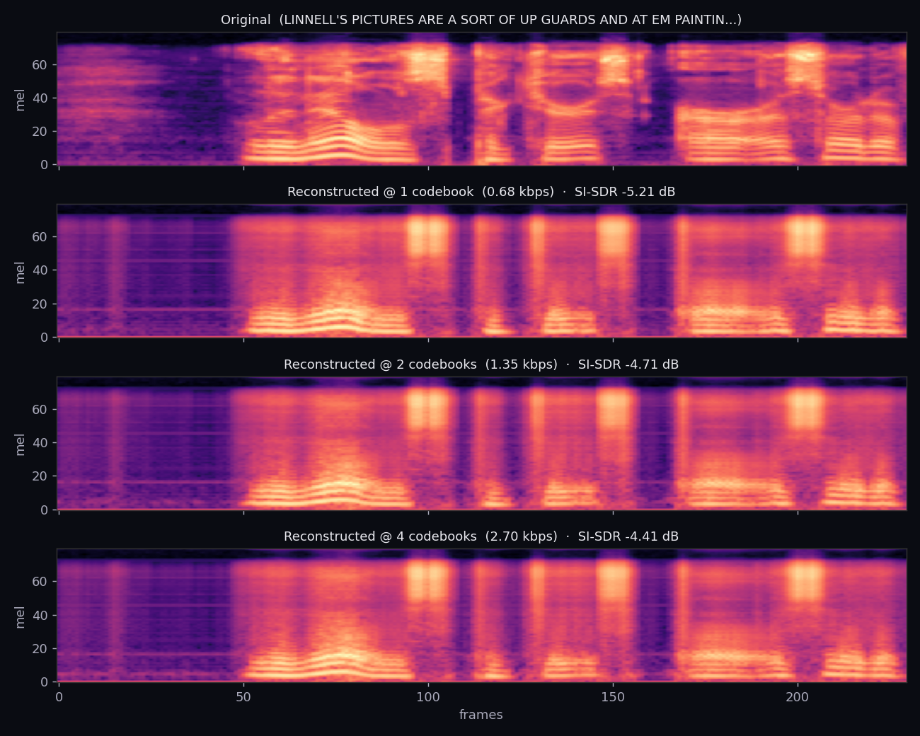
One held-out clip's mel-spectrogram, before and after the codec at each bitrate. As bits drop, fine spectral detail blurs but the harmonic stack and formant trajectories survive — these are the perceptually important parts of speech.

04How it actually works

A neural audio codec compresses a waveform into a sequence of integer codes, then reconstructs it. The whole pipeline is trained end-to-end so the encoder, the discrete bottleneck, and the decoder co-adapt — the codec learns its own representation of audio instead of using a hand-designed one like MP3 or Opus.

05Residual vector quantization, step by step

A single VQ codebook with K entries can represent at most K different points per frame — at 512 entries that's only 9 bits. To squeeze more information out of every frame without raising the frame rate (and the bitrate), residual VQ stacks codebooks: the second codebook quantizes the leftover error from the first, the third quantizes the error from the second, and so on.

# Residual VQ — what each iteration of the loop does
residual = z                            # start with the encoder's continuous latent
out      = zeros_like(z)
for vq in codebooks:               # 4 codebooks here
    # nearest-neighbour lookup in this codebook
    idx = ((residual - vq.codebook) ** 2).sum(-1).argmin(-1)
    q   = vq.codebook[idx]              # the chosen entry
    out      = out + q                  # add it to our running reconstruction
    residual = residual - q             # subtract; whatever is left is the new target
return out, indices                     # `out` ≈ z; `indices` are the integer codes

The encoder output is a continuous vector. The stack of indices is what we transmit (or store, or feed to a downstream language model). The decoder only ever sees out, which is just the sum of codebook entries the indices point to — everything past the encoder is a discrete sequence of small integers.

06One model, three bitrates: quantizer dropout

Notice that in the sample player above, three different reconstructions of the same clip all come from the same model — we just chose to decode using 1, 2, or 4 codebooks. That works because of a small but important training trick from SoundStream and EnCodec: at each training step, we pick a random number of active codebooks and only run that many. The decoder learns to produce a reasonable waveform whether it sees the contribution of one, two, or four codebooks.

for step in range(steps):
    x = next_batch()
    # pick how many codebooks are active for THIS step
    n_active = randint(1, n_codebooks + 1)
    y, _, commit, codebook = model(x, n_active=n_active)
    loss = recon_l1(y, x) + multiscale_stft(y, x) + 0.25 * commit + codebook
    loss.backward(); opt.step()

Without this trick, the decoder would over-rely on the highest codebooks and degrade catastrophically when you tried to use fewer of them. With it, you get a single model with a scalable bitrate dial. That's the property that lets a downstream language model stream at low bitrate and a higher-quality renderer decode at full bitrate.

07Back-propagating through an argmin

The single trickiest part of training any neural codec: the argmin that picks a codebook entry is not differentiable. There's no gradient that tells the encoder "you should have produced a slightly different latent so a different codebook entry was chosen." If we tried to backprop through it honestly, the encoder would never learn.

The straight-through estimator sidesteps the problem with a one-liner: in the forward pass we use the quantized vector q; in the backward pass we pretend the lookup was the identity function — gradients flow from the decoder straight back into the continuous latent z as if nothing had been quantized.

# forward = q (discrete), backward = ∂/∂z is identity
q_st = z + (q - z).detach()

(q - z).detach() is treated as a constant by autograd, so ∂q_st / ∂z = 1. The encoder gets a usable gradient, the decoder only ever sees codebook entries, and the codebook itself is moved towards the encoder outputs by a separate commitment loss — the 0.25 * commit term above.

08Why time-domain L1 isn't enough — the multi-scale STFT loss

A naive choice is to just minimise ‖y − x‖₁ in the time domain. That fails badly for audio: two waveforms can sound identical to a human while being out of phase by a few samples, and the L1 loss will report a huge error. The model would then learn to produce a blurry, over-smoothed signal that minimises pointwise error but sounds awful.

Multi-scale STFT loss compares magnitude spectrograms at several FFT resolutions — we no longer care about phase, only about the energy distribution across frequency at different time scales. Big FFT windows catch the long-term harmonic structure; small windows catch transients and consonants. The codec is rewarded for getting the time-frequency shape right, which is closer to what the human ear actually hears.

def multiscale_stft_loss(y_hat, y):
    return sum(
        stft_loss(y_hat, y, n_fft=n, hop=h)
        for n, h in [(2048, 512), (1024, 256), (512, 128), (256, 64)]
    ) / 4

def stft_loss(y_hat, y, n_fft, hop):
    Y, Yh = stft(y, n_fft, hop), stft(y_hat, n_fft, hop)
    sc       = (Y.abs() - Yh.abs()).norm() / Y.abs().norm()       # spectral convergence
    log_mag  = F.l1_loss(Yh.abs().log(), Y.abs().log())          # log-magnitude L1
    return sc + log_mag

09Are we actually using all the codebook entries?

"Codebook collapse" is a classic failure mode: the encoder lands on a handful of entries and ignores the rest, throwing away the capacity you paid for. The right diagnostic is each codebook's effective perplexity — exp(H(usage)) — which measures the effective number of entries actually being used. For a codebook of size 512, perplexity close to 512 is healthy; close to 1 is collapse.

In a healthy RVQ stack the first codebook usually has the highest perplexity (it sees the raw latent and benefits most from spreading entries out); later codebooks have lower perplexity because the residuals they're quantizing are smaller and more concentrated near zero. Watch for any codebook collapsing below ~50 — that's a sign of a sick training run.

10Why this matters

Discrete audio tokens are the lingua franca of modern generative-audio systems. Every recent speech LM — AudioLM, VALL-E, Moshi, Voicebox, Mimi — sits on top of a neural codec that turns waveforms into integer sequences a transformer can autoregress over. The same architecture appears in:

• Conversational speech-to-speech — Moshi and friends use codec tokens as both input and output of a duplex speech LM.
• Text-to-speech — Voicebox, VALL-E, and Bark generate codec tokens conditioned on text; the codec decoder renders them to audio.
• Speech translation — token-level translation between languages without round-tripping through text.
• Codec-based diffusion — diffusion in the codec latent space instead of raw waveforms.
• Streaming inference — low-bitrate codecs let you run real-time audio over noisy networks at < 3 kbps.

This project is the codec piece, built from the ground up so the joints — strided conv geometry, residual VQ math, the straight-through gradient, quantizer dropout, multi-scale STFT loss, codebook diagnostics — are all visible and modifiable. Drop in a different decoder, a different quantizer, a different loss, and the rest of the pipeline keeps working.